Machine Learning Project

Harmony in Motion: Advancing Yoga Pose Recognition through Machine Learning

Introduction:

The project aims to merge yoga, an ancient practice, with modern machine learning techniques to develop a model for accurately recognizing and classifying yoga postures. Utilizing a comprehensive dataset, the project seeks to enhance the understanding and performance of yoga practices across various skill levels. The project has an experimental approach(trial and error) of testing and comparing techniques of dimensionality reduction, clustering, and diverse classifiers and CNN algorithms for this dataset to develop more robustness and its ability to generalize across different yoga postures.

Data Source:

Sourced from Kaygel, comprising 2,454 annotated yoga posture images, the dataset is robust, meticulously annotated, and represents a wide spectrum of yoga styles, providing a strong foundation for model training and evaluation.

Understanding Dataset:

Type of Target Variable:The target variable remains the yoga posture label, representing specific yoga poses depicted in each image. This categorical target variable contains multiple classes corresponding to different yoga poses. This is a non-linear and multi-class classification problem.
Features Included:The primary features included in the model will be the images of yoga postures. Each image will serve as a feature, with pixel intensity values capturing the visual characteristics of the yoga poses.

Research Question:

How effectively can a machine learning algorithm distinguish and categorize a wide range of yoga postures in images, considering the variability in backgrounds, lighting conditions, and the subtle differences in how individuals perform each pose?

Model Approach:

Fusion Approach: Combines insights from both supervised and unsupervised learning to create a comprehensive model capable of recognizing explicit visual cues and understanding underlying pose variations.
Unsupervised Learning with Clustering: Applies clustering techniques for in-depth pose analysis, exploring patterns and relationships within the data without explicit labels.
Supervised Learning with Transfer Learning and CNNs: Utilizes Convolutional Neural Networks for training on the annotated dataset, incorporating transfer learning to enhance generalization across diverse yoga styles.

Methodology:

Preprocessing and Dimensionality Reduction:

Prepare the data by cleaning, normalizing, and reducing dimensionality to make it suitable for further analysis. Techniques like PCA (Principal Component Analysis) or t-SNE (t-distributed Stochastic Neighbor Embedding) can be employed.

Exploration of Pre-trained Models and Manifold Learning Techniques:

Explore existing pre-trained models and manifold learning techniques to handle the complexity of the dataset. Manifold learning techniques like Isomap can help visualize the data's underlying structure.

Unsupervised Learning with Clustering:

Apply unsupervised learning techniques such as clustering (e.g., K-means, Spectral clustering) to the preprocessed data. This helps identify patterns and relationships within the data without relying on explicit labels.

Clustering Analysis:

Perform clustering analysis using techniques like K-means clustering on features extracted by Isomap or other manifold learning techniques. This step helps uncover inherent patterns and structures within the data.

CNN Model Development with Early Stopping and Learning Rate Scheduling:

Develop a CNN model tailored specifically for yoga pose recognition. Implement techniques like early stopping and learning rate scheduling to prevent overfitting and improve performance.

Supervised Learning with Transfer Learning and CNNs:

Utilize Convolutional Neural Networks (CNNs) for training on the annotated dataset. Transfer learning can be applied to leverage pre-trained models, enhancing generalization across diverse yoga styles.

Model Comparison and Evaluation: Compare the performance of different models developed during the previous steps. Evaluate factors such as accuracy, computational efficiency, and robustness to determine the most effective approach for yoga pose recognition
Methodology Breakdown:
Initial Raw Data Pre-processing :
Observation of the dataset:
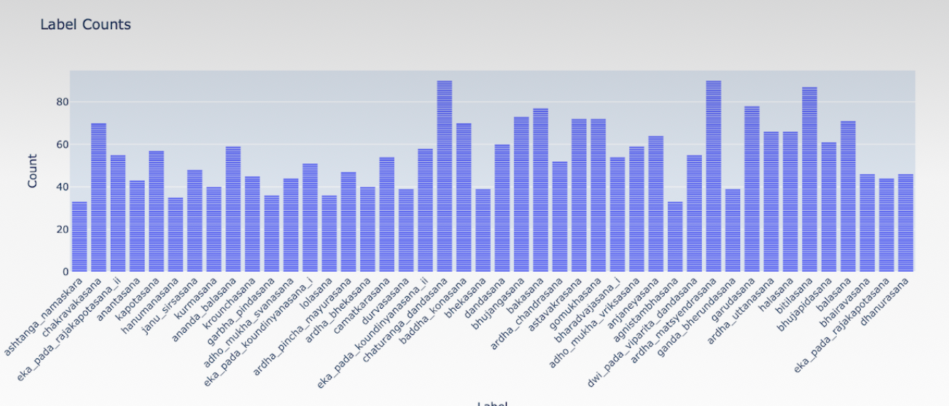
Found 44 different subfolders of images of yoga postures in the main folder.
Subfolders of images were labeled but images within each were not labeled.
Each subfolder had around minimum of 33 to a maximum of 90 images
Images were colored in RGB format
Images had different backgrounds
Images were of different size
Transformed Images into Analyzable Data: Grayscaling and CSV Conversion:
Wrote code for grayscaling of images and converting images into CSV format with two columns of images and labels.
The code used: Code
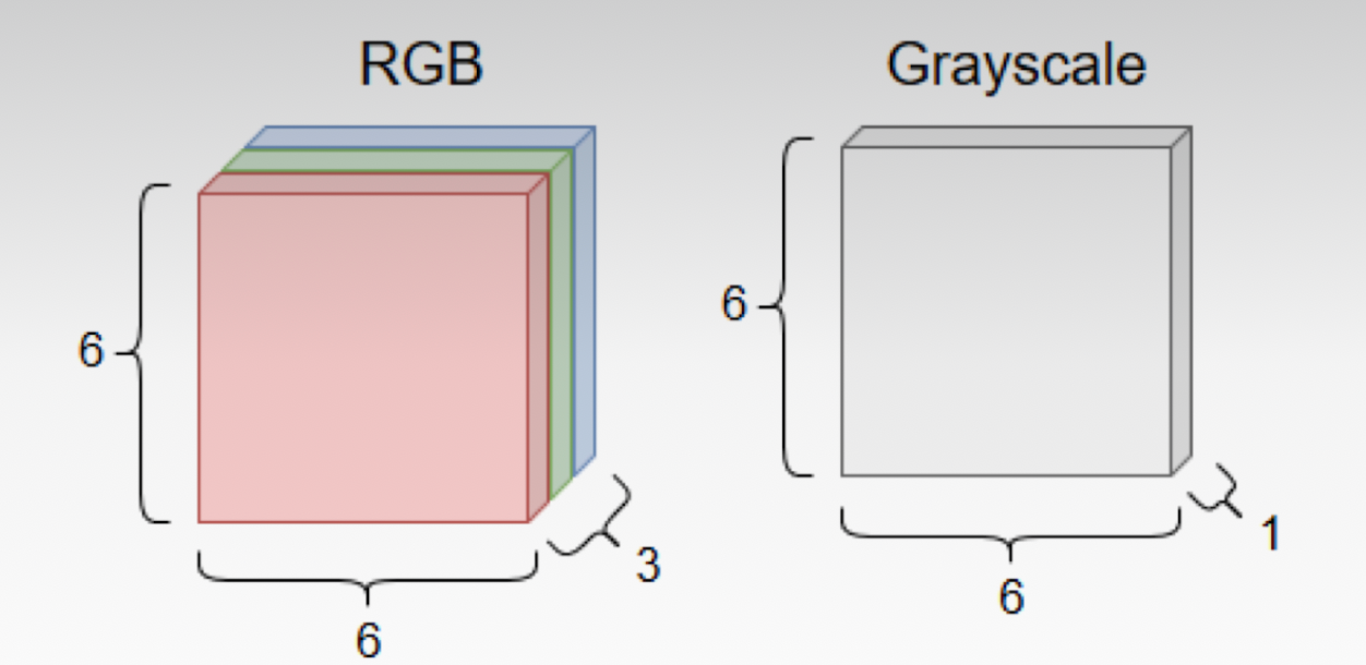
Grayscaling in Machine Learning: Enhancing Image Analysis Efficiency:
Grayscaling simplifies image processing in machine learning by reducing data dimensionality and focusing on texture and shape, leading to faster, more efficient algorithm performance and uniformity across diverse images.

Chose a Platform for Machine Learning: Google Colab:
Uploaded zip files of images and CSV to Gdrive
Mounted Gdrive to Google Colab
Imported necessary libraries
Initial data description before pre-processing:
The shape of the data frame
Summary Statistics
Visualizations of summary statistics: Box Plot, Bar Chart

Made data machine-readable:

# Made the Data Machine Readable

label_encoder = LabelEncoder()

df['encoded_label'] = label_encoder.fit_transform(df['label'])

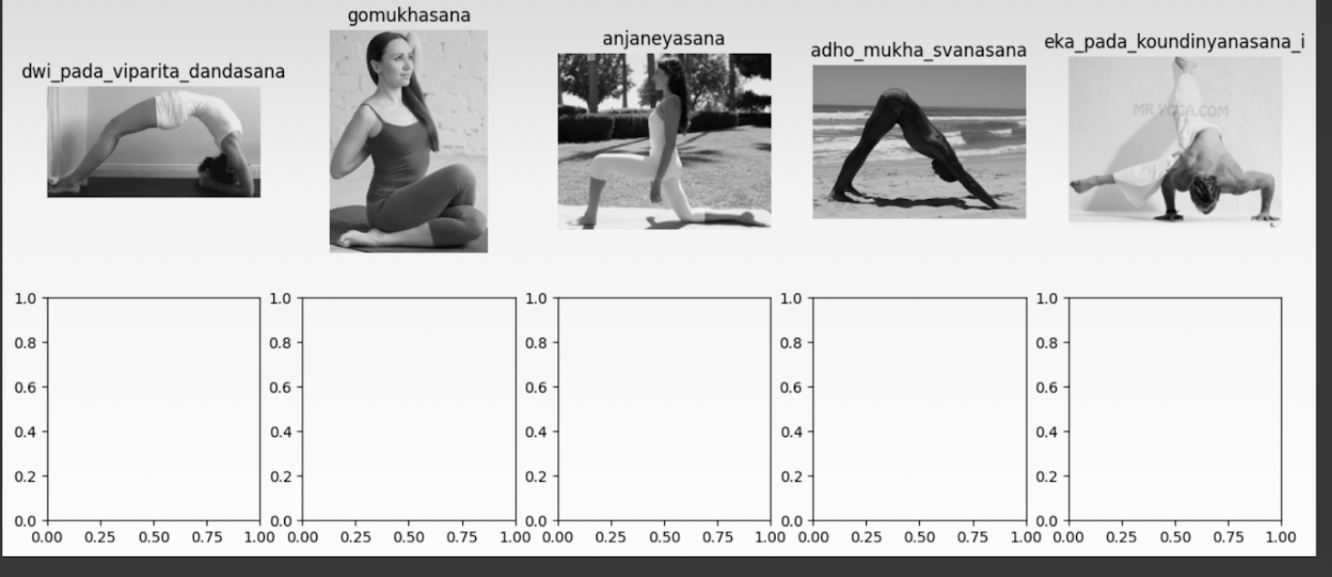
Visualization of images before preprocessing:
Here you’ll see they are in grayscale already, though in different sizes.

Pre-Processing Images:
Resizing images using PIL:
Ensuring consistency in input data dimensions, which is essential for training models efficiently.

One hot encoding/Label Indexing :
Converted one-hot encoded labels to class indices to convert categorical labels (such as class names) into a binary format that models can work with
Each class is represented by a unique binary vector, ensuring that the model does not assume a natural ordering among classes
NumPy arrays:
Converted the unified lists of resized images and corresponding labels into numpy arrays for easier manipulation and processing in subsequent machine-learning tasks.
Splitting of Dataset:
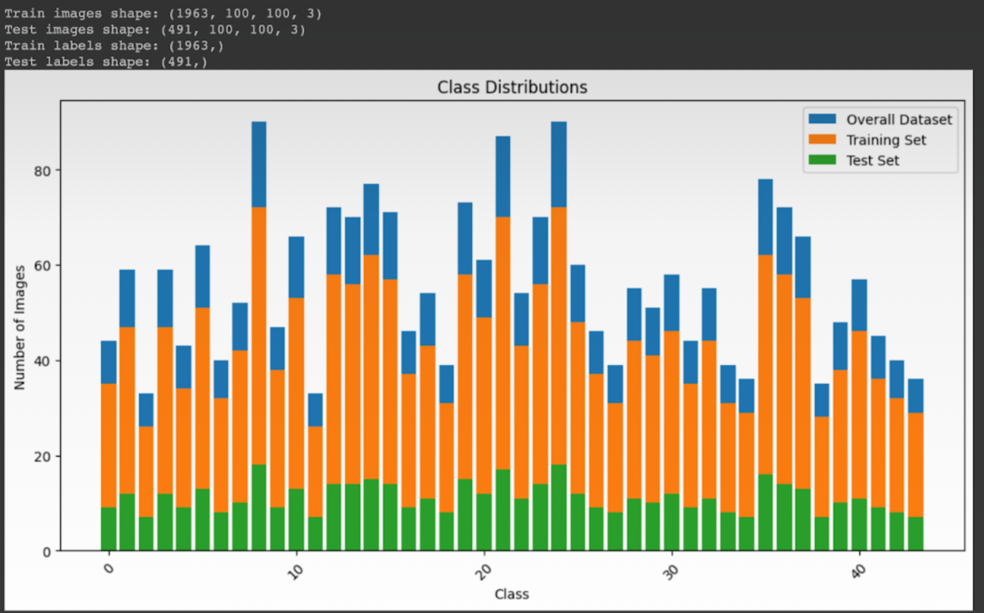
The data is split and verified.
Point to note: Throughout the code, the pixels show up as (100, 100, 3) but to note that images have already been grayscaled and therefore I have deliberately left them in this format, avoiding grayscaling, already grayscale images

Stratified Sampling:
Stratified sampling guarantees that every category of an image, especially classes with fewer images is adequately represented in the test and train datasets.

Manifold learning technique for dimensionality reduction:
Manifold learning techniques are particularly well-suited for non-linear datasets because they can capture the non-linear structure of the data and represent it in a lower-dimensional space while preserving important relationships. Techniques employed for exploring data using training class labels:
Isomaps:
Isomap is well-suited for capturing the overall geometric structure of the data, including both local and global relationships. It tends to preserve the intrinsic geometry of the data and preserves the geodesic distances (shortest path distances) as closely as possible.
The plot shows the data points in a two-dimensional space, where each point represents an image, and the color indicates the class label assigned during unsupervised learning.
Observation: The plot shows multiple colors being mixed, and an overlap between different points indicating that images from different classes are close in the reduced feature space hence signifying difficult classification and a complex data structure.

Laplacian Eigenmaps:
LLE first linearly reconstructs each input point from its nearest neighbors
It is a powerful tool for exploring the intrinsic geometry of the data and preserves local information only.
Observation: The 'U' shape of the distribution indicates that there's a fundamental two-dimensional manifold structure in the high-dimensional data and suggests that the data points are organized in a nonlinear manner.

t-SNE((t-distributed Stochastic Neighbor Embedding):
t-SNE is particularly good at preserving the local structure of data and is a way to check if the image features have been learned in such a way that they form distinct groups based on the training class labels.
Observation: In this t-SNE plot, indicates that while there is some structure to the data, there may be challenges in achieving high classification accuracy due to overlaps and the complexity of the feature space.

UMAP (Uniform Manifold Approximation and Projection):
It is a relatively recent technique that is particularly effective for visualizing clusters or groups within high-dimensional data.
It is flexible and can be applied to a wide variety of data types beyond just numerical data, including categorical, binary, and mixed datasets.
Observation: This particular plot shows tighter clustering compared to the Isomap,t-SNE, plot, which may suggest better class separability. The presence of distinct clusters indicates a meaningful structure in the data that could be leveraged for tasks such as classification.

Conclusion:
From the above visualization, UMAP performed better in preserving both the local and global structure of underlying data and also making tighter clusters than other techniques. Therefore, I decided to do clustering on UMAP features.
Unsupervised learning using UMAP features:
Clustering with k=5 for both K-Means and Spectral Clustering.
K-Means Clustering:
K-means assumes that clusters are convex and isotropic, which means it perform well when the natural clusters in the data are roughly spherical or hyper-spherical.
Silhouette Kmeans Score = 0.41602528
Observation: Silhouette_kmeans score indicates that clustering on the dataset indicates a moderate level of cluster separation and cohesion.

Spectral Clustering :
Designed to identify clusters based on the connectivity of the data points, making it more suited to complex cluster shapes that are not necessarily globular.
Silhouette Spectral Score = 0.3805717
Observation: Silhouette Spectral Score is relatively low in comparison to that of K-Means indicating that clusters are moderately defined, with data points being closer to other points in their cluster than to points in other clusters.

Conclusion:
We see that K means clustering performed better than
Earlier for my metrics score I tried ARI and NMI scores as well, but removed them later as they tend to give incorrect metrics when the number of clusters(k=5) doesn't match the number of true classes(44). Therefore I focused on metrics like the silhouette score, which measures how similar an object is to its cluster compared to other clusters.

Supervised Learning:
Two approaches were taken here:
Testing various classifiers: Naive Bayes, RFM, SVC
Transfer Learning through CNN Models:'CNN', 'MobileNetV2', 'DenseNet121', 'ResNet50', 'VGG19', 'InceptionV3', 'EfficientNetB0'.
Testing various classifiers: Non-Linear Classification:
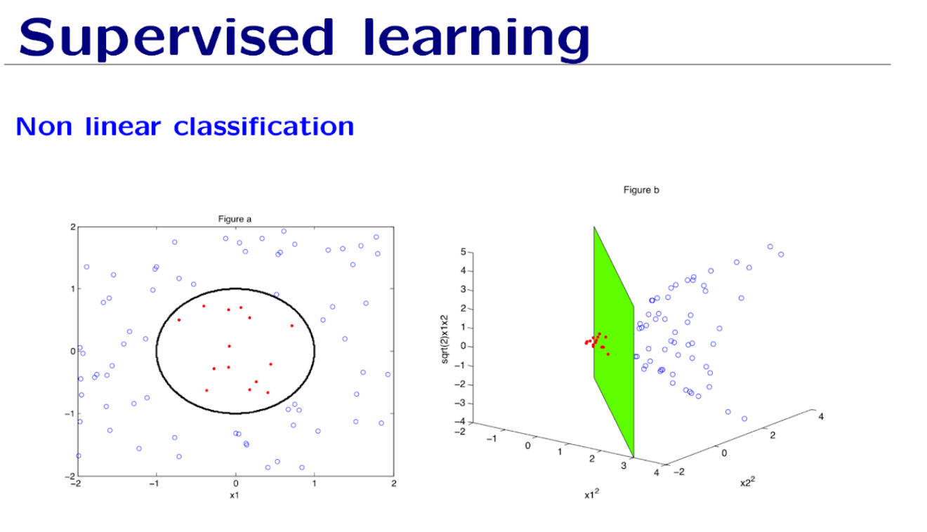
Non-linear classifiers are designed to capture the intricate patterns in data that cannot be separated by a straight line or a linear equation
In the given figures we see the power of kernel methods or feature space transformations in machine learning in non-linear classifiers, where such techniques are used to find a hyperplane in a higher-dimensional space that can linearly separate classes that are not linearly separable in the original space.

Naive Bayes:
Here is a picture of how naive Bayes works:

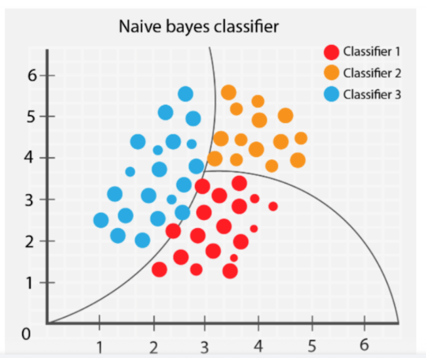
This algorithm is inherently linear because it assumes independence between the features and uses the probability of each attribute belonging to each class to make a prediction. However, in practice, it is used to model complex relationships due to its probabilistic foundation and can work well even when the independence assumption does not hold.
Accuracy Score:0.1955193482688391
Observation: On experimenting with this I received a very low accuracy score of 0.1955193482688391, testifying in a way of the non-linear nature of my dataset. This was not a good approach as pixels in images are highly correlated(non-linear)
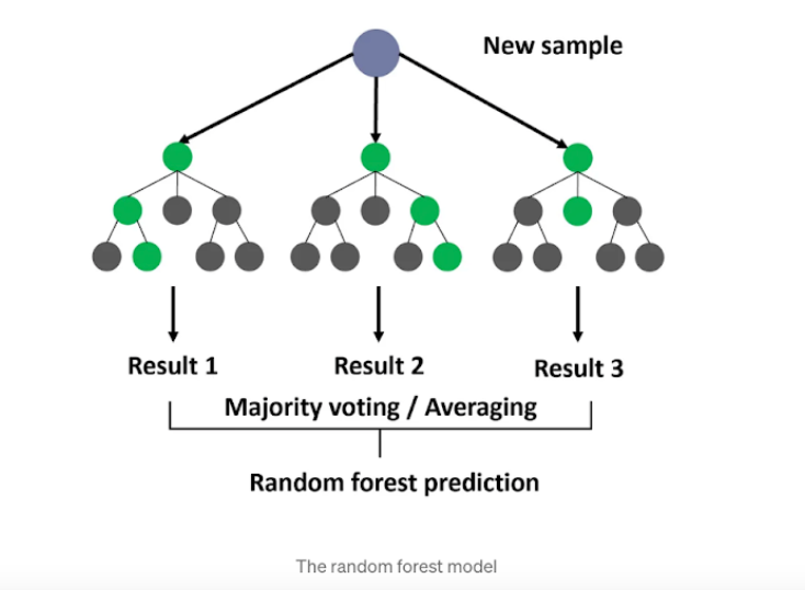
It operates by building multiple decision trees and is intrinsically capable of modeling non-linear relationships without any special transformation of the feature space.
The decision boundaries created by individual trees are non-linear, and when aggregated, they can capture very complex relationships between features and the target variable.

Random Forest:

Accuracy score:0.3340122199592668
Observation: Random forests may not be well-suited for image data due to the high dimensionality and complex relationships between pixels.
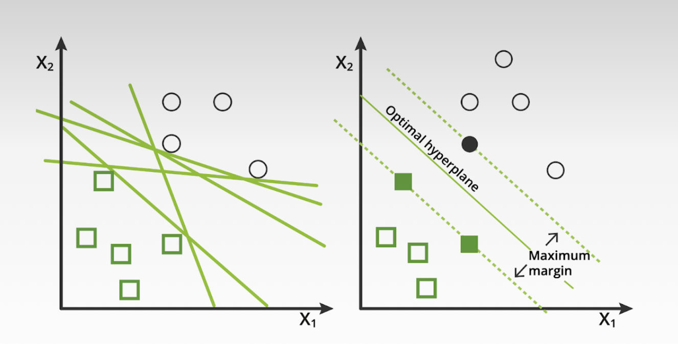
SVMs are versatile in that they can be used for both linear and non-linear classification.
For non-linear classification, SVMs use kernel functions (like the radial basis function, polynomial, or sigmoid kernels) to map the input data into a higher-dimensional space where it becomes linearly separable. This is known as the kernel trick.

SVM:

Accuracy Score: 0.3564154786150713
Observation: SVMs might struggle with low amounts of training data, especially for high-dimensional data like images. Deep learning models often require large amounts of data to generalize well.
Conclusion:
I believe that from this section on using these three classifiers, I learned that the first and foremost important thing is to understand my data type and the independence between the features to apply a specific classifier.
Naive Bayes being a linear classifier gave the lowest score, but I expected specifically SVM to give a better classification score it being almost equal to that of random forest made me dwell more on my image pre-processing steps of feature embedding as well as more number of images for better generalization.
Transfer Learning through CNN Models
Deep Learning CNN Algorithm :
Before getting ahead with specific models and accuracy scores, I wanted to present an understanding of what I learned about the working of a CNN model and its various input and output layers.

Kernel/Filter:
The filter or kernel is one of the functions used in the convolution. The filter will likely have a smaller height and width than the input image and can be considered a window sliding over the image.

Feature Map:
The convolution output is called a feature map. A feature map represents one feature we’re analyzing the image for. We can do padding if we want the size of the feature map to be the same as the image.

Pooling:
Max pooling is good because it maintains important features about the input, reduces noise by ignoring small values, and reduces the spatial size of the problem.

Fully Connected Layers:
Fully connected layers are used to make the final classification in the CNN.
Before moving to the first fully connected layer, we must flatten our input values into a one-dimensional vector that the layer can interpret.
Flattening shows a simple example of converting a multi-dimensional input into a one-dimensional vector.

Activation Function and Output Layer:
The output layer uses some activation function, to convert the neuron values into a probability distribution over our classes. This means that the image has a certain probability of being classified as one of our classes and the sum of all those probabilities equals one.
Why CNNs are best suited for image classification?
Hierarchical Feature Learning:
- CNNs automatically learn hierarchical representations of features from raw pixel values. They consist of multiple layers, including convolutional layers, pooling layers, and fully connected layers, which learn increasingly abstract features as information flows through the network.
Translation Invariance:
- CNNs are inherently translation invariant, meaning they can recognize patterns in images regardless of their location a result, CNNs can detect features irrespective of their position in the image, making them robust to variations in object position and orientation.
Local Receptive Fields:
- Convolutional layers in CNNs utilize local receptive fields, where each neuron is connected to a small region of the input image. capturing local patterns and spatial dependencies within the image, enabling it to learn features such as edges, textures, and shapes effectively.
Parameter Sharing:
- CNNs leverage parameter sharing, where the same set of weights (filters) is used across different spatial locations of the input image. This sharing of parameters reduces the number of learnable parameters in the network and encourages the network to learn spatially invariant features. Consequently, CNNs can efficiently learn from large amounts of image data while avoiding overfitting.
Nonlinear Activation Functions:
- CNNs employ nonlinear activation functions such as ReLU (Rectified Linear Unit) after each convolutional and fully connected layer. These nonlinearities allow the network to learn complex, nonlinear relationships between features in the data, enabling it to model the intricate patterns present in images.
Variants of CNN employed in the model (Transfer Learning):
Basic CNN model:
A simple CNN model can be tailored to the specific needs of your task without the complexity of pre-designed architectures.
It provides the freedom to experiment with the number of layers, filter sizes, and other hyperparameters.

Accuracy Score before:0.21687597773654387
Accuracy Score after: 0.49694502353668213
Observation:
Earlier I got an even lower score of 0.21, but then I increased the epochs=20 and also used dropout with a rate of 0.5, early stopping, and, reduced learning rate by 0.1 hence, receiving a better score of 0.49.
However basic CNNs do not capture as complex features as advanced architectures, which might be one of the reasons for lower accuracy and performance on difficult image classification tasks.
MobileNetV2:
It is designed for mobile and resource-constrained environments.
It is highly efficient in terms of computation and memory, which makes it fast and suitable for applications that need to be run on devices with limited resources, like smartphones and embedded systems.

Accuracy Score:0.5193482637405396
Observation:
- Unlike the basic CNN model, the gap between training and validation accuracy is less pronounced, suggesting that this model is generalizing better than the basic CNN model.
- However, both accuracies plateau towards the end of the epochs, which may suggest that longer training wouldn't necessarily lead to significantly better performance on the validation set.
- There can be various other reasons for low scores MobileNetV2 is pre-trained on ImageNet, which contains a wide range of images, but my yoga posture images are subtle and are different in style, composition, or quality from those in ImageNet, the transfer learning may not be as effective.
DenseNet121:
Each layer in DenseNet is connected to every other layer in a feed-forward fashion, which can lead to improved feature propagation and feature reuse.
Dense connections can lead to a large increase in memory usage, which might be a problem for deep networks or deployment on devices with limited memory.

Accuracy Score before early stopping:0.939393937587738
Accuracy Score before after stopping: 0.969696998596191
Observation:
- There is a steep increase in both training and validation accuracy during the initial epochs, indicating that the model is quickly learning from the data.
- After epoch 4, the training accuracy remains high while the validation accuracy dips and then slightly recovers.
- Therefore, I employed early stopping to it and got an increase, the accuracy score being now: 0.9696969. But again I saw that there is a dip in validation accuracy after epoch 5, hence the model before early stopping might be a better model as it gets plateaus.
ResNet50:
ResNet50 uses residual connections to enable the training of very deep networks by allowing gradients to flow through the network directly. This can lead to very high performance on a variety of image classification tasks.

Accuracy Score: 0.9545454382896423
Observation:
- There is a small and consistent gap between the training and validation accuracy, suggesting that the model is generalizing well without a large amount of overfitting. The validation accuracy appears relatively stable after the initial increase.
- After around epoch 4, both accuracies show stability, indicating that additional training epochs may not result in significant gains in accuracy.
VGG19:
VGG19 has a very uniform architecture that makes it easy to understand and implement. It is often used as a feature extractor for other tasks due to its effectiveness in capturing image features.
Disadvantages: It is quite large and slow to train compared to more modern architectures, and it has a lot of parameters, which makes it computationally intensive to run and prone to overfitting.

Accuracy Score before early stopping:0.9242424368858337
Accuracy Score after early stopping:0.7878788113594055
Observation:
- There is a consistent gap between the training and validation accuracy.It plateaus from epoch two inwards This gap suggests that the model may not generalize as well to unseen data as it does to the training data, again pointing towards overfitting.
- But I tried early stopping and the results worsened, as we can see in the plot therefore the earlier model seemed to be a better choice for my dataset.
InceptionV3:
InceptionV3 uses multiple-sized convolutional filters within the same layer to capture features at various scales.
Disadvantages: The Inception model can be complex to understand and modify due to its sophisticated architecture, and it may still be relatively heavy for resource-constrained environments.

Accuracy Score before early stopping: 0.7727272510528564
- Accuracy Score after early stopping: 0.7727272510528564
Observation:
- The gap between the training and validation accuracy suggests overfitting, where the model performs well on the training data but does not perform equivalently on the validation data.
- I employed early stopping to stop training around epoch 3 or 4, as the validation accuracy does not show significant improvement beyond these epochs.
- To my surprise, the score accuracy score remained the same indicating no significant change, in the plot we see that the distance between train and validation accuracy remains the same.
EfficientNetB0:
EfficientNetB0 utilizes a compound scaling method, scaling up the depth, width, and resolution of the network in a balanced way. It is designed to achieve high accuracy while being efficient regarding parameters and computation.
Disadvantages: While EfficientNet is designed for efficiency, the scaling method requires careful tuning, and it might not always outperform other specialized models for specific tasks.

Accuracy Score before early stopping and learning rate scheduler: 0.21212121844291687
Accuracy Score after early stopping and learning rate scheduler:0.1818181872367859
Observation:
- Despite the early stopping and learning rate scheduler, the model may still be overfitting. This is suggested by the large gap between training and validation accuracy.
- To address this I tried early stopping but the results worsened and the other possible reasons for low validation accuracy could also be a result of a small validation set, noisy labels, or classes that are not well represented.
Model Evaluation Metrics:
Accuracy: Measures the proportion of true results (both true positives and true negatives) among the total number of cases examined.
Precision: Measures the proportion of true positive results in the set of all positive predictions made.
Recall: Measures the proportion of true positive results in the set of all actual positives.
F1 Score: The harmonic mean of precision and recall, providing a balance between them for uneven class distributions.

The effectiveness of the model was measured using four parameters:

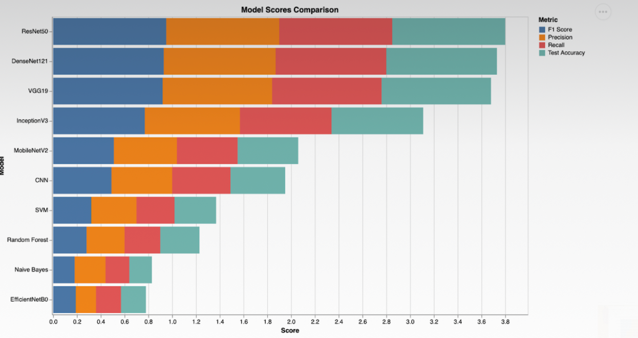
Performed ANOVA F statistics on the accuracy scores of different models and reached the top 3 models most suitable for classification of the yoga posture image dataset.
The top three models selected based on accuracy scores are:
1. ResNet50
2. DenseNet121
3. VGG19
Conclusion(Answering the Research Question):
Each model has their specific advantages and disadvantages.
Implying the importance of architectural features
Each of these models has distinct architectural features that contribute to their success in image classification tasks:
ResNet50 uses residual connections to solve the vanishing gradient problem, allowing for the training of very deep networks without performance degradation.
DenseNet121 employs densely connected layers, where each layer is connected to every other layer in a feed-forward fashion. This architecture leads to improved feature propagation and reuse, making it highly efficient and reducing the risk of overfitting.
VGG19 is characterized by its simplicity, using a series of convolutional layers with small receptive fields followed by max-pooling layers. Despite its simplicity, VGG19 has shown a deep capacity for feature extraction in images.
For my dataset, I found that ResNet50 worked the best, primarily due to its ability to use residual connections to enable the training of very deep networks by allowing gradients to flow through the network directly.
In conclusion, the successful application of CNN models to classify yoga postures amidst various challenges the variability in yoga poses, the background complexity, or the need to capture subtle features- demonstrates the potential of advanced deep-learning models to tackle complex image classification tasks.
It highlights the CNN model's ability to learn detailed features and generalize across different conditions, making it a powerful tool for recognizing and categorizing images with high accuracy, even in the face of significant variability.
OUTLOOK:
The approach to the model has been experimental, and I have tried various diverse algorithms to train, test, and observe which works better
Throughout the model, I have made sure to add respective observations and conclusions to each section along with respective scores for a deeper and more comprehensive understanding of the model.
KEY TAKEAWAYS: I would like to mention that I struggled with a lot of aspects of model making initially but they helped me take away some fundamental learnings for future ML projects:
Understanding the unique needs of a dataset.
Using platforms like Google Collab made my work easier as I did not have to worry about specific libraries working with my local environment or not.
Sometimes I faced issues in running my code due to a lack of dependencies or variables, so I had to do a lot of copy and paste of full codes in many code blocks for running diverse models as I made my model over one month.
Consistent guidance and discussion from peers and Professors were so helpful in mending my model, discussion helped me a lot check my model approach.
Classroom slides were my core guiding principles for building my model effectively.
Understanding that nothing is pre-defined in ML it’s an evolving process in which different results change future paths respectively. For instance, I learned through working with my data that contouring, data augmentation and flattening did not give good results for my dataset.
It is a trial and error, of playing around alternatives to see what works.
While choosing different classifiers and models I had to do my research based on my dataset, which made things easier I knew it was a multiclassification problem and my dataset was non-linear, these two things made my work easier in choosing pre-trained models.
While running CNN models for the second run, I witnessed how different regularization techniques at times transform the accuracy results and sometimes they don’t again point to the unique needs of each dataset.
Understanding the importance of metrics was one of the most crucial learnings to uncover the metrics for each algorithm, I did not wish to base my understanding of visualizations on my conjectures, I wanted them to be based on certain numbers like metrics, therefore helping me lead the way forward each step on as solid foundation.
I understood that ML needs both a comprehensive understanding of theory as well as practice to understand what works better.
I learned the role of different fine-tuning techniques in the betterment of a model.
Each model has their specific advantages and disadvantages.
The potential biases in my dataset in yoga pose recognition can stem from a dataset's lack of diversity in practitioner representation and pose variability, as well as inconsistencies in image backgrounds, quality, and annotation precision.

There is a lot of room for improvement in the model if I had more time, I would have tried various other algorithms and techniques for fine-tuning other models which did not give good accuracy scores for my dataset.